Dengue Exercise 1 Static

In [4]:
import numpy as np
import random
import matplotlib.pyplot as plt
import statsmodels.api as sm
import seaborn as sns
import pylab as pl
get_ipython().magic('matplotlib inline')
from datetime import datetime as dt
import pandas as pd
import sklearn
from sklearn import linear_model
from sklearn import feature_selection
from sklearn.feature_selection import SelectKBest
from sklearn.metrics import mean_squared_error
from sklearn.cross_validation import KFold
sns.set_style("whitegrid")

/Users/galwachtel/anaconda/lib/python3.6/site-packages/statsmodels/compat/pandas.py:56: FutureWarning: The pandas.core.datetools module is deprecated and will be removed in a future version. Please use the pandas.tseries module instead.
  from pandas.core import datetools
/Users/galwachtel/anaconda/lib/python3.6/site-packages/sklearn/cross_validation.py:44: DeprecationWarning: This module was deprecated in version 0.18 in favor of the model_selection module into which all the refactored classes and functions are moved. Also note that the interface of the new CV iterators are different from that of this module. This module will be removed in 0.20.
  "This module will be removed in 0.20.", DeprecationWarning)

In [2]:
#A function built to organize data; this is later replaced with a pandas dataframe. 
def dengue_incidence_searches(f):    
    with open(f) as file:
        dengue_searches=[]   
        dengue_cdc=[]
        dates=[]
        for l in file:
            line=l.strip()
            if line: 
                l=[x for x in l.split()]
                dates.append(str(l[0]))
                dengue_searches.append(float(l[2]))
                dengue_cdc.append(float(l[1]))
    return(dengue_searches, dengue_cdc, dates)

In [3]:
dengue_data=dengue_incidence_searches('Dengue_trends_AM_111_training.txt')
dates=[dt.strptime(l, '%m/%d/%y') for l in dengue_data[2]]

a. Plotting dengue incidence

In [4]:
fig=plt.figure(figsize=(10, 5))
ax=fig.add_subplot(111)
x=dates
y=dengue_data[1]
ax.plot(x, y, 'k')
pl.xlabel('Date')
pl.ylabel('CDC - Cases')
pl.title('Dengue - training data 2004-2006')
pl.show()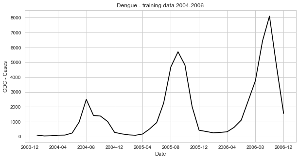

b. Fitting a linear regression using ols

In [5]:
#A function which runs an OLS regression and returns its parameters:
def fitOLS(xval, yval):
    ols=sm.OLS(yval, sm.tools.add_constant(xval)).fit()
    b,a=ols.params
    return (b, a)

In [6]:
Slope, Error = fitOLS(dengue_data[0], dengue_data[1])
print('Slope:', Slope, 'Error:', Error)

Slope: 2155.25181371 Error: 2926.37898735

c.

In [64]:
#Predicting dengue cases form the ols parameters:
b=fitOLS(dengue_data[0], dengue_data[1])[0]
a=fitOLS(dengue_data[0], dengue_data[1])[1]
predicted_dengue_0406=[x*b+a for x in dengue_data[0]]
dates=[dt.strptime(l, '%m/%d/%y') for l in dengue_data[2]]

In [8]:
fig=plt.figure(figsize=(10, 5))
x=dates
y=dengue_data[1]
plt.plot(x, y, 'k', label='CDC cases')
plt.plot(x, predicted_dengue_0406, label='ols static 1')
pl.xlabel('Date')
pl.ylabel('Dengue cases')
pl.title('Dengue - Prediction 2004-2006')
pl.legend(loc='upper left', prop={'size':15})
pl.show()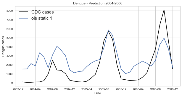

d. Prediction of dengue incidence using ols – with training set

In [9]:
dengue_data_2007_2011=dengue_incidence_searches('Dengue_trends_AM_111_prediction.txt')

In [10]:
predicted_dengue_2007_2011=[x*b+a for x in dengue_data_2007_2011[0]]
dates=[dt.strptime(l, '%m/%d/%y') for l in dengue_data_2007_2011[2]]

In [11]:
fig=plt.figure(figsize=(10, 5))
ax=fig.add_subplot(111)
x=dates
y=dengue_data_2007_2011[1] 
ax.plot(x, y, 'k', label='CDC cases')
ax.plot(x, predicted_dengue_2007_2011, label='ols static 1')
pl.xlabel('Date')
pl.ylabel('Dengue cases')
pl.title('Dengue Static ols (pred:2007-2011) - 1 Var')
pl.legend(loc='upper left', prop={'size':15})
pl.show()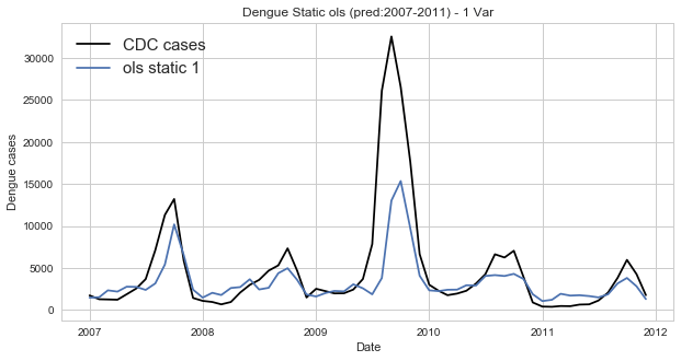

The major flaw of using OLS fpr prediction of dengue incidence is that we are trying to model data which is clearly nonlinear by using a linear model. By examining the training data set we are able to see that dengue incidence is cyclical and clealy not linear. Thus using maximum likelihood would possibly yield a tigghter prediction as it is more suited for nonlinear data. In addition, calculating the parameters in smaller increments, i.e. dynamically, should yield a tighter fit.